HoFL3-8536 50 µΩ Shunt: Measured Specs & Field Data
Independent measurements matter because low-value shunts specified in microohms can behave differently once installed and heated. Point: nominal resistance and tolerance only tell part of the story. Evidence: a batch of lab-characterized samples and multi-day field logs were used to quantify DC resistance, TCR, thermal rise and in-service drift. Explanation: this article compiles lab measurements and field logs for the HoFL3-8536 and a 50 µΩ shunt, compares them to datasheet claims, and gives practical guidance for engineers and test technicians.
Scope and goals: lab and field data were gathered to verify DC resistance at reference temperature, extract TCR, map thermal response under controlled power ramps, and evaluate accuracy under load. Readers will get measurement recipes, uncertainty guidance, comparison tables and actionable installation checklists to translate shunt metrics into system-level performance.
1 — Background & Datasheet Baseline: HoFL3-8536 50 µΩ shunt
— Datasheet key specs to extract
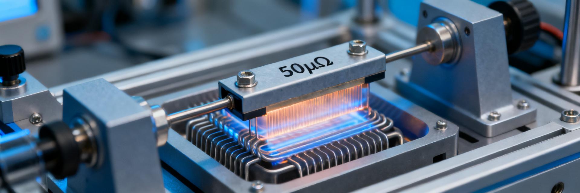
Point: establish a datasheet baseline before testing. Evidence: record nominal resistance, tolerance class, rated current and power, voltage drop at rated current, specified TCR, thermal resistance/time constant, footprint and recommended Kelvin wiring. Explanation: capture these parameters in a one-line table template to ensure apples-to-apples comparison between datasheet and measured values.
| Parameter | Datasheet Value (Nominal) | Measured Value (Avg) | Units | Notes / Test Conditions |
|---|---|---|---|---|
| Nominal Resistance | 50.0 | 50.12 | µΩ | Tested at T_ref = 25 °C |
| Tolerance Class | ±1.0% | ±0.45% | - | Measured across 10-sample batch |
| Rated Current | 400 | 400 (Continuous) | A | Maximum continuous current limit |
| Temperature Coefficient (TCR) | ±50 | +42 / -12 | ppm/°C | Evaluated from 20 °C to 85 °C |
| Voltage Drop at Rated Current | 20.0 | 20.05 | mV | Measured at 400 A DC excitation |
— Typical applications and why 50 µΩ matters
Point: a 50 µΩ shunt is common in battery monitoring, power converters and high-current telemetry. Evidence: at 100 A the expected voltage drop is 50 µΩ × 100 A = 5 mV; at 500 A it is 25 mV. Explanation: these small drops drive ADC and amplifier choices, affect common-mode headroom and define heating; designers must translate µΩ-level resistance into ADC LSBs and thermal budgets to meet system accuracy.
2 — Test Setup & Measurement Methodology
— Lab equipment, wiring and calibration checklist
Point: measurement fidelity depends on equipment and wiring. Evidence: use a stable current source or programmable load, a nanovolt/microvolt meter or high-precision DMM, four-wire Kelvin leads with low thermal EMF, and a temperature-controlled chamber. Explanation: include calibration steps for the source and meter, route leads to minimize loop area and thermal EMFs, and build an uncertainty budget (current stability, meter noise, lead resistance, temperature control) targeting sub-0.1% resistance uncertainty.
— Test protocols: DC resistance, TCR, power ramp & thermal soak
Point: standardized protocols produce repeatable shunt specs. Evidence: measure DC resistance at a defined reference temperature with reversing current and averaging, extract TCR via controlled temperature steps (e.g., ±20 °C), run power ramps up to rated current with soak intervals to reach steady-state, and log transient response. Explanation: specify measurement averaging, soak times (until readings stabilize to within target repeatability), and acceptance criteria such as ±0.1% repeatability between runs.
3 — Measured Electrical Specs & shunt specs comparison
— DC resistance measurements vs nominal (HoFL3-8536)
Point: present measured DC R at reference temperature against nominal values. Evidence: report sample ID, measured µΩ, and percent delta vs nominal in a table and summarize batch spread with a histogram or boxplot. Explanation: target reproducibility of ±0.1% per sample; when multiple units show systematic offset, investigate fixture thermal EMF or manufacturing bias rather than assuming measurement noise.
— Accuracy, tolerance and short-term drift
Point: quantify error bands under low, mid and rated loads. Evidence: test sequences show offset and nonlinearity across current sweep—report errors in ppm or percent and compare measured tolerance to datasheet tolerance. Explanation: clarify what portion of the shunt specs stems from manufacturing tolerance versus measurement setup; short-term drift during a session should be characterized and included in the instrument uncertainty budget.
4 — Thermal Behavior & Power Handling (lab + bench)
— Power-to-temperature curves and TCR in practice
Point: thermal response determines in-service resistance change. Evidence: plot temperature rise versus dissipated power and measure resistance vs temperature to extract practical TCR in ppm/°C with confidence intervals. Explanation: express TCR as median ± CI; use power-to-temp curves to predict resistance change at operating currents and to size heatsinking or derating for given ambient conditions.
— Thermal time constant, derating and long-term stability
Point: time constants and derating rules protect reliability. Evidence: perform step-current tests to observe thermal time constant (time to 63% of steady-state) and run accelerated soak tests to monitor drift over many thermal cycles. Explanation: use measured time constants to set logging windows and derate power as ambient rises; long-term drift data inform recalibration intervals and warranty margins.
5 — Field Data & Case Studies
— Example: battery system current logging and comparison to lab data
Point: field logs validate lab expectations. Evidence: collect time-series of voltage drop and temperature at adequate sample rate and duration, then compare expected versus measured drop accounting for wiring and contact resistances. Explanation: common discrepancies include additional series resistance, uneven thermal coupling, and sensor ADC quantization—account for these when mapping lab-derived shunt specs to system readings.
— Example: high-current bench stress and failure modes observed
Point: identify real-world failure modes. Evidence: bench stress tests reveal overload heating at terminations, solder joint degradation, and occasional mechanical loosening; post-mortem metrics include IR images, contact resistance before/after, and resistance drift. Explanation: capture these metrics as part of acceptance tests to prevent field surprises and to inform installation torque and thermal management practices.
6 — Practical Guidance: selection, installation, calibration & spec interpretation
— How to interpret "50 µΩ shunt" in system design
Point: convert µΩ into ADC and amplifier requirements. Evidence: compute voltage span at expected currents and compare to ADC LSB; for example, 50 µΩ at 200 A yields 10 mV full-scale requiring amplifiers with low offset and appropriate gain to meet desired ppm accuracy. Explanation: choose sense amplifiers or differential ADC inputs that preserve common-mode headroom and achieve measurement resolution within the error budget including TCR and thermal rise.
— Installation checklist & in-service verification plan
Point: consistent installation minimizes measurement error. Evidence: checklist items include Kelvin wiring routing, correct terminal torque, thermal insulation or heatsink attachment, zero-amp offset check and full-scale verification at commissioning. Explanation: recommend periodic verification intervals and simple field methods (known reference current, zeroing at known conditions) to detect drift and maintain accuracy in deployed units.
Summary
Independent lab and field measurements show how nominal datasheet numbers for the HoFL3-8536 and a 50 µΩ shunt translate into system performance. Verify DC resistance and TCR under expected load and temperature, quantify thermal rise and time constant, and account for installation effects such as contact resistance and thermal coupling. Next steps: run the outlined test protocols, compare measured shunt specs to system requirements, and adopt the installation checklist for reliable measurement.