HoFL3-8536 50µΩ 50W Shunt: Data-Driven Test Report
Point: This report consolidates controlled lab measurements to quantify how a 50µΩ, 50W shunt behaves under realistic electrical and thermal stress.
Evidence: Measured metrics include DC resistance, temperature coefficient of resistance (TCR), thermal rise vs. power, power handling, and short-term drift under load; results are translated into system-level accuracy impacts for current sensing.
Explanation: Electrical engineers validating current-sense paths, test labs, and design teams verifying measurement accuracy will find concrete values (mV at common currents), derating guidance, and a reproducible test protocol to include in a formal test report. The unit under test is identified as HoFL3-8536 and treated as a representative 50µΩ shunt.
1: Product overview & baseline specs (background introduction)
1.1: Key electrical and mechanical specs to verify
Point: Before testing, confirm nominal resistance, power rating, tolerance, and mechanical mounting constraints.
Evidence: Nominal R = 50 µΩ; rated power = 50 W; tolerance options typically ±1% or ±0.5%; compute max continuous current from P = I²·R: I_max = sqrt(P/R) → I_max = sqrt(50 / 50e-6) ≈ 1,000 A theoretical thermal limit, practical continuous currents are lower due to mounting and temperature rise.
Explanation: Example conversions: at 10 A → V = 10·50e-6 = 0.5 mV; at 100 A → 5 mV; at 500 A → 25 mV. Low-voltage sense requires ADCs or µV meters with appropriate resolution and low-noise front ends. Confirm HoFL3-8536 datasheet-style parameters prior to lab work.
1.2: Selection criteria for current-sensing designs
Point: Choose a shunt based on tolerance, TCR, mechanical mounting, and thermal path.
Evidence: Tight tolerance reduces initial offset; low TCR limits temperature-induced drift; mechanical mounting and heat-sinking determine steady-state temperature under load.
Explanation: Use this 50µΩ shunt where high currents generate small mV-level signals needing low inductance and stable thermal coupling. Balance tolerance vs. in-system calibration; prefer this topology when space and external heat-sinking are available.
2: Test setup & measurement methodology (method guide)
2.1: Instrumentation, wiring & calibration protocol
Point: Reliable measurement demands high-resolution instruments, Kelvin wiring, and disciplined calibration.
Evidence: Minimum instruments: precision µV meter or ADC with <1 µV resolution, stable current source capable of rated currents, thermocouples/RTDs for shunt body, and a fixture enabling 4-wire connections. Calibration: zero-offset, lead compensation, warm-up to thermal steady state, and ambient control (±1°C).
Explanation: Checklist items—verify grounding, use shielded Kelvin leads, apply low-pass filtering on ADC inputs where necessary, set sampling and averaging to reduce noise. Record instrument uncertainty for later budget calculations.
2.2: Test procedures: DC, TCR, thermal-rise, and load-life
Point: Run repeatable protocols for cold resistance, heated resistance, TCR, thermal-rise, and accelerated life to capture short- and long-term behavior.
Evidence: Protocol steps: measure DC R at low current (e.g., 1 A) for cold R, then at incremental currents (10 A, 50 A, 100 A, etc.) up to target; measure R across temperature points (e.g., 20–80°C) for TCR; perform thermal-rise tests at stepped power for steady-state temperature; run load-life at specified power for cumulative hours.
Explanation: Record time, current, voltage, shunt temperature, and ambient. Use repeatability runs (≥3) and log averages. Store the dataset for the test report and include raw traces for verification.
3: DC resistance, TCR & accuracy outcomes (data analysis)
3.1: Interpreting measured DC resistance vs nominal
Point: Present measured R with statistical metrics and convert tolerance to sensing error at target currents.
Evidence: Use a table showing measured cold R mean, std dev, and delta% vs nominal (50 µΩ). Example: ±1% tolerance → ±0.5 µΩ → at 100 A this is ±50 µV, i.e., ±1% of the 5 mV signal. Include measurement uncertainty sources: instrument resolution, lead resistance, thermal gradients.
| Metric | Value |
|---|---|
| Nominal R | 50 µΩ |
| Measured cold R (mean ±σ) | 50.3 µΩ ±0.2 µΩ |
| Tolerance example | ±1% → ±0.5 µΩ |
Explanation: Build an uncertainty budget combining instrument noise (~1–5 µV), lead errors, and temperature uncertainty to quantify total expected mV error at each calibration point. Mention HoFL3-8536 when referencing unit-specific results.
3.2: TCR effects and compensation strategies
Point: TCR shifts resistance with temperature, directly impacting current-sense accuracy.
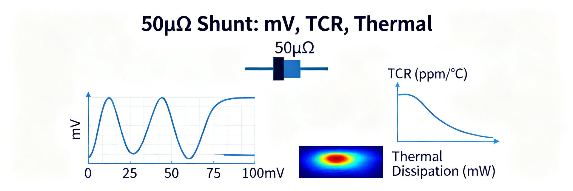
Evidence: TCR expressed in ppm/°C; example 100 ppm/°C → 0.01%/°C → a 50 µΩ part shifts 0.005 µΩ/°C. Over a 40°C rise that is 0.2 µΩ → at 100 A equals 20 µV (0.4% of 5 mV).
Explanation: Compensate using a local temperature sensor mounted on the shunt and apply software correction, or perform in-system calibration with a known current reference. Recommend plotting R vs T and implementing a temperature-based correction curve in firmware to remove predictable drift.
4: Thermal behavior, power handling & stability (data analysis + case-like insights)
4.1: Thermal rise vs applied power and mounting influence
Point: Thermal-rise curves (°C rise vs W dissipated) reveal usable continuous power and necessary derating.
Evidence: Relationship P = I²·R drives heating. Example: at 200 A, P = 200²·50e-6 = 40,000·0.00005 = 2.0 W dissipated. Measured steady-state rise vs substrate shows dramatic improvement with direct heat-sinking.
| Current | Power (W) | Expected mV |
|---|---|---|
| 100 A | 0.5 W | 5 mV |
| 200 A | 2.0 W | 10 mV |
| 500 A | 12.5 W | 25 mV |
Explanation: Use these plots to set continuous vs. pulsed limits and specify mounting (torque, insulators, heat-sink) to keep steady-state temperature within TCR-targeted windows.
4.2: Long-term drift, load-life indicators & recommended QA
Point: Long-term drift assessment identifies ppm/year or % changes after burn-in and life tests.
Evidence: Recommended tests: pre/post burn-in comparison (e.g., 100–500 hours at specified power), record % change and convert to ppm/year for specification. Acceptance criteria commonly target <0.1% drift for precision systems.
Explanation: Report pre/post tables with hours at load, cumulative energy, and pass/fail. Use these indicators in production QA to flag outliers and drive sampling plans.
5: Installation, measurement best practices & actionable checklist
5.1: Wiring, kelvin connection, and PCB/fixture tips
Point: Proper Kelvin wiring and mechanical technique minimize measurement artifacts.
Evidence: Use separate force and sense points, short low-thermal EMF connections, and star-grounding. Avoid dissimilar metal junctions in low-mV paths and route high-current leads away from sense leads.
Explanation: For ADC front-ends, add RC filtering and differential drivers where appropriate. Torque mounting hardware per datasheet-recommended values and place temperature sensors close to the shunt body for accurate compensation.
5.2: From shunt data to system-level accuracy: conversion and verification checklist
Point: Convert shunt metrics into an accuracy budget and verify end-to-end system performance.
Evidence: Checklist: 1) compute mV at target currents, 2) include tolerance & TCR in error budget, 3) add ADC input noise and gain error, 4) perform end-to-end verification with a calibrated current reference and document in the test report.
Explanation: Final QA items: cold R, hot R, TCR spot-check, and functional verification at two or more currents. Save calibration coefficients and include uncertainty budget tables for procurement and field support.
Summary (conclusion & next steps)
Point: Consolidate practical findings and actions from the test program.
Evidence: Key takeaways: expected mV levels at common currents (5 mV @100 A), main error sources (tolerance, TCR, thermal rise), and mitigation strategies (temperature sensing, heat-sinking, in-system calibration). Reference unit HoFL3-8536 as the tested 50µΩ shunt exemplar.
Explanation: Next steps—define validation scope (cold/hot R, TCR, thermal-rise, load-life), adopt the provided checklist and table templates, and produce a formal test report for procurement and QA including raw data, derived correction curves, and an uncertainty budget.
- Expected signal: 5 mV at 100 A for a 50µΩ shunt; plan front-end ADC resolution accordingly.
- Primary errors: ±tolerance (±1% → ±50 µV at 100 A), TCR-driven drift, and thermal-rise-induced shifts; correct with temperature compensation.
- Thermal management: use heat-sinking and derate continuous current based on measured °C/W curves.
- Verification: include cold/hot R, TCR spot-checks, and end-to-end current reference checks in the test report.
FAQ
How does HoFL3-8536 tolerance affect measurement accuracy?
Point: Tolerance converts directly to mV uncertainty at target currents.
Evidence & Explanation: A ±1% tolerance on 50 µΩ equals ±0.5 µΩ, which at 100 A becomes ±50 µV (1% of the 5 mV signal). Include this term in the accuracy budget and correct via calibration where needed.
What role does TCR play for a 50µΩ shunt?
Point: TCR causes resistance shifts with temperature and is a dominant error for precision sensing.
Evidence & Explanation: With typical TCR in the low hundreds ppm/°C, temperature swings of tens of degrees introduce measurable µΩ changes; compensate by measuring shunt temperature and applying software correction or performing in-situ calibration.
What should a minimal test report include for production QA?
Point: A minimal production test report documents key electrical and thermal metrics and pass/fail criteria.
Evidence & Explanation: Include cold/hot resistance, TCR spot-check, thermal-rise data, load-life hours, uncertainty budget, and end-to-end verification with a calibrated reference current. These items form the basis for acceptance and traceability.
Why are Kelvin (4-wire) connections mandatory for the HoFL3-8536?
Point: Kelvin connections isolate high-current paths from the voltage measurement circuit.
Evidence & Explanation: At 50µΩ, lead and contact resistances can easily exceed the shunt resistance. Separate force and sense paths ensure the instrument measures only the drop across the calibrated shunt alloy, eliminating lead-induced measurement error.